Секрет 2 (Ускоряем GROUP BY)
Обычный GROUP BY при наличии большого числа метрик можно ускорить, используя CTE, также снизив размер спилла
Secret 2(Speed up GROUP BY)
Simple GROUP BY operator with a lot of aggregates can be boosted using CTE (cutting spill usage as well)
Обычный GROUP BY при наличии большого числа метрик можно ускорить, используя CTE, также снизив размер спилла
Secret 2(Speed up GROUP BY)
Simple GROUP BY operator with a lot of aggregates can be boosted using CTE (cutting spill usage as well)
--sub-optimal code:
select dim1, dim2, dim3, sum(m1), sum(m2), ..., sum(m50)
from foo
group by 1, 2, 3

--good code
with a as
         (select dim1, dim2, dim3, sum(m1), sum(m2), ..., sum(m25)
          group by 1, 2, 3),
     b as
         (select dim1, dim2, dim3, sum(m26) m26_agg, sum(m27) m27_agg, ..., sum(m50) m50_agg
          group by 1, 2, 3)
select a.*, b.m26_agg, b.m27_agg, ..., b.m50_agg
from a, b
where a.dim(1, 2, 3) = b.dim(1, 2, 3) -- краткая форма записи для join-а по всем измерениям /  short form of a.dim1 = b.dim1 and ... and a.dim3 = b.dim3
🔥1
Секрет 3 (Вездесущая статистика)
Частой причиной зависания запроса и/или генерации спилла является отсутствие статистики по таблицам запроса.
Если ваш ETL основан на PL/pgSQL функциях, то режимом сбора статистики ( если не задан на уровне GUC - Global User Configuration )
рулит параметр gp_autostats_mode_in_functions, который должен быть установлен в самой функции ( не до ее вызова )
Secret 3 (Omnipresent statistics)
A common reason for a query to hang and/or generate a spill is the lack of statistics on the query tables.
If your ETL is built on PL/pgSQL functions, then the statistics gather mode ( if not set by GUC - Global User Configuration )
is managed by gp_autostats_mode_in_functions parameter which must be set in the function itself ( otherwise it doesn't matter )
CREATE OR REPLACE FUNCTION public.fn_foo()
RETURNS boolean
LANGUAGE plpgsql
AS $function$
    begin
      set gp_autostats_mode_in_functions = on_no_stats; -- безуслловный сбор статистики по таблицам, модифицируемым в функции / always gather stat for all tables modified by function
  -- Другие значения / other values:
  --   none - не собирать статистику / don't gather stat,
  --   on_change - собирать статистику если число измененных записей превысило заданный порог  / gather stat if  the number of modified records exceeds specified threshold
  ...
👍3🔥1
Секрет 4 (Осторожно - Рекурсия!)
Следует избегать рекурсивных запросов , т.к. join таблицы с ней же несовместим с концепцией shared-nothing.
Иными словами, такая операция приводит к тиражированию таблицы на каждый узел класера, т.к.
не может выполняться локально (только на своем) ввиду распределения таблицы только по одному из ключей предиката запроса.
Однако, если join-ить таблицу не саму на себя ( рапределенную по AGREEMENT_PK в примере ниже), а с ее копией, распределенной по PREVIOUS_AGREEMENT_PK( 2е плечо предиката),
размер спилла можно заметно сократить на порядок.
Secret 4 (Beware - Recursion!)
Recursive queries should be avoided, because joining a table with itself is incompatible with the shared-nothing concept.
In other words, such an operation leads to replicating the table to each cluster node, because it cannot be performed locally (only on its own) due to the distribution of the table only by one of the keys of the query predicate.
However, If you join the table not to itself (distributed by AGREEMENT_PK in the example below), but with its copy distributed by PREVIOUS_AGREEMENT_PK (the parent key in the predicate),
the size of the spill can be significantly reduced by an order of magnitude.
-- bad code
with recursive
                                agreement_chain as
                                (

                                select
                                    AGREEMENT_PK,
                                    PREVIOUS_AGREEMENT_PK,
                                    counter_rec,
                                from foo
                                where is_first_agreement = 'y'
                                union all
                                select
                                    t1.AGREEMENT_PK,
                                    t2.AGREEMENT_PK as PREVIOUS_AGREEMENT_PK,
                                    t2.counter_rec + 1,
                                from foo t1
                                inner join  agreement_chain t2  on t2.AGREEMENT_PK = t1.PREVIOUS_AGREEMENT_PK
                                                                and t2.counter_rec < 10 -- ограничение по рекурсии чтобы не уйти в бесконечный цикл / limitation on recursion to avoid an infinite loop

                                )

                                select
                                    AGREEMENT_PK,
                                    PREVIOUS_AGREEMENT_PK
                                from agreement_chain

-- good code
create table foo_mirror as select * from foo distribued by (PREVIOUS_AGREEMENT_PK);

with recursive
                                agreement_chain as
                                (

                                select
                                    AGREEMENT_PK,
                                    PREVIOUS_AGREEMENT_PK,
                                    counter_rec,
                                from foo
                                where is_first_agreement = 'y'
                                union all
                                select
                                    t1.AGREEMENT_PK,
                                    t2.AGREEMENT_PK as PREVIOUS_AGREEMENT_PK,
                                    t2.counter_rec + 1,
                                from foo_mirror t1
                                inner join  agreement_chain t2  on t2.AGREEMENT_PK = t1.PREVIOUS_AGREEMENT_PK
                                                                and t2.counter_rec < 10

                                )

                                select
                                    AGREEMENT_PK,
                                    PREVIOUS_AGREEMENT_PK
                                from agreement_chain
Секрет 5 (Join без ключа)
Еще один пример потенциальной бомбы - это запросы без '=' в предикате соединения таблиц,
в частности такой, где используется операция between в join-е таблиц без ключа, которая в GP выполняется крайне неоптимально ( через Nested Loop, а не через быстрый Hash Join )
Например, если в таблице продаж foo отсутствует ключ измерения dim_periods, прямое решение в лоб вытащить период для каждой строки foo - это ловушка.
Однако, если в foo уровень детализации данных - день,
то в общем случае число строк будет на порядки больше числа дней, в которые были продажи и
в таком случае ловушки можно избежать, приведя запрос к форме equi-join:
Secret 5(Non-Equi Join)
Another example of a potential bomb is queries without '=' in the table join predicate.
Particularly, one that uses the between operation in a join of tables without a key, which in GP is performed extremely suboptimally (through Nested Loop, and not through fast Hash Join)
For example, if the sales table foo is missing the dim_periods dimension key, a straight forward solution to pull out period for each row of foo is a trap.
However, if foo has a data granularity of day,
then in the general case the number of rows will be orders of magnitude greater than the number of days in which there were sales and
in this case, the pitfall can be avoided by transforming the query in equi-join form:
--bad code (метод соединения/ join method - Nested Loop )
select foo.*, d.date_from, d.date_to
from foo
         join dim_periods d on
    foo.dt between d.date_from d.and date_to


--good code ( вместо NL оптимизатор использует в итоге  Hash Join / Instead of NL optimizer finally uses Hash Join )
with a as
(select distinct dt from foo),
x as ( a.dt, s.* from dim_periods s, a
where a.dt between s.date_from s.and date_to ) -- используем NL лишь для малой доли от foo / use NL path only for tiny % of foo

select foo.*, x.date_from, x.date_to
from foo join x on foo.dt = x.dt
👍3
Секрет 6 (Проблема пустой таблицы, ч.2)
Секрет 1 поведал нам, что select из пустой таблицы может подвисать, создавая спилл.
Оказывается, запрос использующий пустую таблицу в качестве фильтра, по которой нет статистики может создать те же проблемы.
В примере ниже используется реальный кейс в крупном DWH на сотни TB где идет select из интерфейсной функции по диапазону дат с фильтрацией по пустой таблице.
Сбор статистики по пустой таблице foo решает проблему.
К слову, в идеале, не стоит злоупотреблять использованием функций вместо таблиц в запросах, т.к. в этом случае используется Legacy optimizer от Postgres,
а не нативный GPORCA
Secret 6 (Empty table problem, part 2)
Secret 1 told us that select from an empty table can hang, creating a spill.
It turns out that a query using an empty table as a filter for which there are no statistics can also fall into the same problem.
The example below uses a real case in a large DWH for hundreds of TB, where there is a select from an interface function by a range of versions with filtering by an empty table.
Collecting statistics on an empty table foo solves the problem.
By the way, ideally, you should avoid the use of functions instead of tables in queries, because in this case the Legacy optimizer from Postgres is used, and not the native GPORCA.
select deal_rk
      from fn_foo( p_dt_from :='2024-09-01', p_dt_to :='2024-09-02')
      where 1 = 1
        and src_cd = 'IMOEX'
        and coalesce(add_info_04, '&&&') not like '%NON_RESIDENT%'
        and id in (select risk_contract_id from foo) -- плохой фильтр если даже таблица пустая, но без статистики / bad filter if even the table is empty but without statistics
👍3
Секрет 7(Боливар не выдержит двоих или проблема перекоса)
На днях словили на проде неочевидную ошибку при left join 2х таблиц совершенно обычных для нашего ХД размеров
При этом аналогичный запрос с inner join отрабатывает без проблем :
Secret 7 (Bolivar can't bring two or the problem of skew)
Recently we caught a non-obvious error in production when left joining 2 tables of completely normal sizes for our data warehouse.
At the same time, a similar query with inner join works without problems:
Вскрытие показало, что в таблице small_tbl половина ключей оказались NULL + addr_fk является ключом распределения в таблице.
Проблему решили малой кровью, заменив left join объединением двух множеств:
The analysis showed that in the small_tbl table half of the keys were NULL + addr_fk is the distribution key in the table. The problem was solved with little effort by replacing left join with a union of two sets:
На днях словили на проде неочевидную ошибку при left join 2х таблиц совершенно обычных для нашего ХД размеров
При этом аналогичный запрос с inner join отрабатывает без проблем :
Secret 7 (Bolivar can't bring two or the problem of skew)
Recently we caught a non-obvious error in production when left joining 2 tables of completely normal sizes for our data warehouse.
At the same time, a similar query with inner join works without problems:
-- bad query
select a.*, b.address
from small_tbl a -- 7 млн строк ( 7 mln rows )
LEFT JOIN big_tbl b -- 1 млрд строк ( 1 bln rows )
on a.addr_fk = b.addr_pk
ERROR: Canceling query because of high VMEM usage.

-- friendly query
select a.*, b.address
from small_tbl a JOIN big_tbl b
on a.addr_fk = b.addr_pk
Вскрытие показало, что в таблице small_tbl половина ключей оказались NULL + addr_fk является ключом распределения в таблице.
Проблему решили малой кровью, заменив left join объединением двух множеств:
The analysis showed that in the small_tbl table half of the keys were NULL + addr_fk is the distribution key in the table. The problem was solved with little effort by replacing left join with a union of two sets:
select a.*, b.address
from small_tbl a
left join big_tbl b
on a.addr_fk = b.addr_pk
where a.addr_fk is not null
union all
select a.*, null
from small_tbl a
where a.addr_fk is null
Секрет 8(Сколько весит таблица .. или о добром cross-join замолвите слово!)
Как-то наш DBA подготовил отчет о размере таблиц по требуемому списку и крайне удивился.
Оказалось, что функция pg_relation_size для вычисления размера таблицы дает разный результат в зависимости от контекста ее использования.
Проведем простой эксперимент
Secret 8 (How much does a table weigh... or say a word about a good cross-join!)
Once our DBA prepared a report on the size of tables for the required list and was extremely surprised.
It turned out that the pg_relation_size function for calculating the size of a table gives different results depending on the context of its use.
Let's conduct a simple experiment
Определим размер : Let's determine its size:
Это корректный результат.
Создадим список из 1 элемента с названием таблицы выше
This is the correct result.
Let's create a list of 1 element with the table name above
Определим размер таблиц списка: Let's determine its size:
Как же так ?
Дело в том, что запрос показывает размер на том сегменте, где лежит строчка с ее названием в public.foo_2.
Решением в лоб будет join cписка c pg_class
The point is that the query shows the size of the public.foo part on the segment where the line with its name in public.foo_2 is located.
The straightforward solution would be to join the list with pg_class
Однако оно не самое оптимальное, т.к. сильно нагружает каталог.
Существует более элегантный вариант, который стоит смело брать на вооружение.
However, it is not the most optimal, as it heavily loads the catalog.
There is a more elegant option that is A MUST!
Как-то наш DBA подготовил отчет о размере таблиц по требуемому списку и крайне удивился.
Оказалось, что функция pg_relation_size для вычисления размера таблицы дает разный результат в зависимости от контекста ее использования.
Проведем простой эксперимент
Secret 8 (How much does a table weigh... or say a word about a good cross-join!)
Once our DBA prepared a report on the size of tables for the required list and was extremely surprised.
It turned out that the pg_relation_size function for calculating the size of a table gives different results depending on the context of its use.
Let's conduct a simple experiment
create table public.foo   WITH (appendonly=true,orientation=column,compresstype=zstd,compresslevel=1)
as select generate_series(1,1000000) n;
Определим размер : Let's determine its size:
SQL> select pg_relation_size('public.foo')

pg_relation_size
------------------------------
3 209 024 байт
Это корректный результат.
Создадим список из 1 элемента с названием таблицы выше
This is the correct result.
Let's create a list of 1 element with the table name above
create table public.foo_2
as select 'public.foo'::text as tbl_nm;
Определим размер таблиц списка: Let's determine its size:
SQL> select pg_relation_size(tbl_nm) from public.foo_2

pg_relation_size
------------------------------
4 640 байт
Как же так ?
Дело в том, что запрос показывает размер на том сегменте, где лежит строчка с ее названием в public.foo_2.
Решением в лоб будет join cписка c pg_class
The point is that the query shows the size of the public.foo part on the segment where the line with its name in public.foo_2 is located.
The straightforward solution would be to join the list with pg_class
select pg_relation_size(t.tbl_nm) from
pg_class c, pg_namespace s, public.foo_2 t
where 1=1
and s.oid = c.relnamespace
and s.nspname || '.' || relname = t.tbl_nm
Однако оно не самое оптимальное, т.к. сильно нагружает каталог.
Существует более элегантный вариант, который стоит смело брать на вооружение.
However, it is not the most optimal, as it heavily loads the catalog.
There is a more elegant option that is A MUST!
SQL> select sum(pg_relation_size(y.tbl_nm || decode(q.content, q.content, '')))
from public.foo_2 y
cross join gp_dist_random('gp_id') q

sum
------------------------------
3 209 024 байт
👍2
Forwarded from MarketTwits
🔥1
Forwarded from MarketTwits
Секрет 9(Осторожно сиквенс!)
Как-то мне поручили аудит DWH на сотни TB, точнее его etl потоков.
В выгрузке в стэйж из источника для генерации уникального ключа строки
было обнаружено массовое использование сиквенсов, своего в каждом потоке.
Для архитекторов у меня теперь было 2 новости - плохая и хорошая.
Плохая в том, что сиквенсы использовались некэшированные, а это - дорогое удовольствие.
Проведем эксперимент.
Secret 9 (Beware of sequence!)
Once I was assigned to audit DWH for hundreds of TB, or rather its etl streams.
In the unloading to stage from the source for generating a unique row key,
massive use of sequences was discovered, one for each stream.
For architects, I now had 2 news - bad and good.
The bad news is that sequences were used uncached, and this is an expensive pleasure.
Let's conduct an experiment.
А теперь сгенерируем 1 млн значений сиквенса, использующего кэш.
Now let's generate 1 million sequence values using the cache.
1й вариант медленнее в 190 раз!
Но есть нюанс.
Если вам нужен диапазон ключей без дырок, то быстрый вариант подойдет не всегда
Проверим этот факт, запросив сиквенс в двух разных сессиях.
Option 1 is 190 times slower!
But there is a nuance.
If you need a range of keys without holes, then the fast option will not always work
Let's check this fact by requesting a sequence in two different sessions.
Также, стоит отметить, что на каждый созданный сиквенс выделяется место, например в нашем кластере из 720 нод он весит 23 MB.
Таким образом, если под каждый поток или etl выгрузку создается новый сиквенс без его последующего удаления,
что имело место в нашем DWH ( Don't ask me - why ), то это плохое проектирование, плата за которое очень высока.
В рамках моего аудита я обнаружил 737 000 таких зомби весом в 15 TB, что также засоряет и каталог.
Also, it is worth noting that space is allocated for each created sequence, for example, in our cluster of 720 nodes it weighs 23 MB.
Thus, if a new sequence is created for each stream or etl unload without its subsequent deletion,
which was the case in our DWH (Don't ask me - why), then this is bad design, the price for which is very high.
As part of my audit, I found 737,000 such zombies weighing 15 TB, which also clutters the catalog.
Как-то мне поручили аудит DWH на сотни TB, точнее его etl потоков.
В выгрузке в стэйж из источника для генерации уникального ключа строки
было обнаружено массовое использование сиквенсов, своего в каждом потоке.
Для архитекторов у меня теперь было 2 новости - плохая и хорошая.
Плохая в том, что сиквенсы использовались некэшированные, а это - дорогое удовольствие.
Проведем эксперимент.
Secret 9 (Beware of sequence!)
Once I was assigned to audit DWH for hundreds of TB, or rather its etl streams.
In the unloading to stage from the source for generating a unique row key,
massive use of sequences was discovered, one for each stream.
For architects, I now had 2 news - bad and good.
The bad news is that sequences were used uncached, and this is an expensive pleasure.
Let's conduct an experiment.
create sequence public.sq_1;

create table public.sq_1_tst
as select nextval('public.sq_1') sq, generate_series(1,1000000) n;
1,000,000 rows affected in 3 m 11 s 203 ms
А теперь сгенерируем 1 млн значений сиквенса, использующего кэш.
Now let's generate 1 million sequence values using the cache.
create sequence public.sq_1000 cache 1000;

create table public.sq_1000_tst
as select nextval('public.sq_1000') sq, generate_series(1,1000000) n;
1,000,000 rows affected in 1 s 156 ms
1й вариант медленнее в 190 раз!
Но есть нюанс.
Если вам нужен диапазон ключей без дырок, то быстрый вариант подойдет не всегда
Проверим этот факт, запросив сиквенс в двух разных сессиях.
Option 1 is 190 times slower!
But there is a nuance.
If you need a range of keys without holes, then the fast option will not always work
Let's check this fact by requesting a sequence in two different sessions.
SQL> select pg_backend_pid(), nextval('public.sq_1000')
pg_backend_pid | nextval
---------------+--------
11309          | 1001001

SQL> select pg_backend_pid(), nextval('public.sq_1000')
pg_backend_pid | nextval
---------------+--------
12208          | 1002001
Также, стоит отметить, что на каждый созданный сиквенс выделяется место, например в нашем кластере из 720 нод он весит 23 MB.
Таким образом, если под каждый поток или etl выгрузку создается новый сиквенс без его последующего удаления,
что имело место в нашем DWH ( Don't ask me - why ), то это плохое проектирование, плата за которое очень высока.
В рамках моего аудита я обнаружил 737 000 таких зомби весом в 15 TB, что также засоряет и каталог.
Also, it is worth noting that space is allocated for each created sequence, for example, in our cluster of 720 nodes it weighs 23 MB.
Thus, if a new sequence is created for each stream or etl unload without its subsequent deletion,
which was the case in our DWH (Don't ask me - why), then this is bad design, the price for which is very high.
As part of my audit, I found 737,000 such zombies weighing 15 TB, which also clutters the catalog.
❤3👍1
Секрет 10( Ускоряем count(distinct) )
Наверное многие знают, что подсчет уникальных значений - одна из самых дорогих операций для БД
Однако, оказывается, зачастую ее можно ускорить.
Например, если надо посчитать count(distinct) по полю, входящему в хэш таблицы,
у меня для вас хорошие новости.
Существует альтернатива, не требующая больших доработок кода- все, что нужно знать - ключ распределения таблицы,
в которой считаем уникальные кортежи.
Синтезируем датасет из 1 млрд триплетов, который и будет его хэшом , в 3 шага.
Создадим 1000 уникальных значений
Secret 10 (Speeding up count(distinct))
Many people probably know that counting unique values is one of the most expensive operations for a database.
However, it turns out that it can often be accelerated.
For example, if you need to calculate count(distinct) by a field included in the table hash, I have good news for you.
There is an alternative that does not require major code modifications - all you need to know is the distribution key of the table,
in which we count unique tuples.
We synthesize a dataset of 1 billion triplets, which will be its hash, in 3 steps.
Let's create 1000 unique values
Размножим его до 1 млн строк (1000 x1000):
Let's multiply it to 1 million rows (1000x1000):
Ради интереса проверим, сколько уникальных n2 получилось ?
For the sake of interest, let's check how many unique n2 we got?
select count(distinct n2) from public.tst2 -- 248 083 ( А вы думали 1 млн Did you think 1 million? )
И наконец размножим сет до 1 млрд строк ( 1 000 000 x 1000 ), не забыв про ключ распределения:
And finally, we will multiply the set to 1 billion rows (1,000,000 x 1000), not forgetting about the distribution key
Для тех, кому понравился предыдущий чек, уникальных значений n3 получилось 32 136 768
Проверим число строк в итоговом датасете
For those who liked the previous check, the unique values of n3 were 32,136,768.
Let's check the number of rows in the final dataset
и его хэш and its hash
Все готово для гонок.
Замерим старый добрый подход
All set for racing.
Let's measure the good old school approach
И альтернативу, где используется дедупликация для подачи в count уже уникального набора
And we'll run an alternative that uses deduplication to feed count with an already unique set
Если глянуть на explain analyze на фото, то можно заметить, что планы почти одинаковы, но в быстром варианте (справа) есть дополнительный Agregate,
который делается на нодах и только потом сокращенная выборка пересылается на мастер (Gather Motion), где идет финальный подсчет числа элементов.
Будем считать, что на фото выполнен повторный прогон бенчмарка в режиме explain analyze, где быстрый вариант показал почти то же самое время, а традиционный сильно ускорился, но все равно в 7 раз медленнее.
If you look at the explain analyze in the photo, you can see that the plans are almost the same..
Наверное многие знают, что подсчет уникальных значений - одна из самых дорогих операций для БД
Однако, оказывается, зачастую ее можно ускорить.
Например, если надо посчитать count(distinct) по полю, входящему в хэш таблицы,
у меня для вас хорошие новости.
Существует альтернатива, не требующая больших доработок кода- все, что нужно знать - ключ распределения таблицы,
в которой считаем уникальные кортежи.
Синтезируем датасет из 1 млрд триплетов, который и будет его хэшом , в 3 шага.
Создадим 1000 уникальных значений
Secret 10 (Speeding up count(distinct))
Many people probably know that counting unique values is one of the most expensive operations for a database.
However, it turns out that it can often be accelerated.
For example, if you need to calculate count(distinct) by a field included in the table hash, I have good news for you.
There is an alternative that does not require major code modifications - all you need to know is the distribution key of the table,
in which we count unique tuples.
We synthesize a dataset of 1 billion triplets, which will be its hash, in 3 steps.
Let's create 1000 unique values
create table public.tst1   WITH (appendonly=true,orientation=column,compresstype=zstd,compresslevel=1)
as select generate_series(1,1000) n1;
Размножим его до 1 млн строк (1000 x1000):
Let's multiply it to 1 million rows (1000x1000):
create table public.tst2   WITH (appendonly=true,orientation=column,compresstype=zstd,compresslevel=1)
as select t1.n1, t1.n1*t2.n1 n2 from
public.tst1 t1, public.tst1 t2
Ради интереса проверим, сколько уникальных n2 получилось ?
For the sake of interest, let's check how many unique n2 we got?
select count(distinct n2) from public.tst2 -- 248 083 ( А вы думали 1 млн Did you think 1 million? )
И наконец размножим сет до 1 млрд строк ( 1 000 000 x 1000 ), не забыв про ключ распределения:
And finally, we will multiply the set to 1 billion rows (1,000,000 x 1000), not forgetting about the distribution key
create table public.tst3   WITH (appendonly=true,orientation=column,compresstype=zstd,compresslevel=1)
as select t1.n1, t1.n2, t1.n2*t2.n1 n3  from
public.tst2 t1, public.tst1 t2
distributed by (n1,n2,n3);
Для тех, кому понравился предыдущий чек, уникальных значений n3 получилось 32 136 768
Проверим число строк в итоговом датасете
For those who liked the previous check, the unique values of n3 were 32,136,768.
Let's check the number of rows in the final dataset
SQL> select reltuples from pg_class c, pg_namespace s where relname = 'tst3'
and s.nspname = 'public'
and s.oid = c.relnamespace;
reltuples
--------------
1 000 000 000
и его хэш and its hash
SQL>select pg_get_table_distributedby('public.tst3'::regclass)
pg_get_table_distributedby
------------------------------------------
DISTRIBUTED BY (n1, n2, n3)
Все готово для гонок.
Замерим старый добрый подход
All set for racing.
Let's measure the good old school approach
SQL>select count(distinct n1)  from  public.tst3
count
--------
1 000
execution: 6 m 30 s 459 ms
И альтернативу, где используется дедупликация для подачи в count уже уникального набора
And we'll run an alternative that uses deduplication to feed count with an already unique set
SQL> select count(*)
from (
         select n1
         from (
                  select n1, n2, n3
                  from dbg.tst3
                  group by 1, 2, 3) a
         group by 1) b;
count
---------
1 000
execution: 15 s 386 ms
Если глянуть на explain analyze на фото, то можно заметить, что планы почти одинаковы, но в быстром варианте (справа) есть дополнительный Agregate,
который делается на нодах и только потом сокращенная выборка пересылается на мастер (Gather Motion), где идет финальный подсчет числа элементов.
Будем считать, что на фото выполнен повторный прогон бенчмарка в режиме explain analyze, где быстрый вариант показал почти то же самое время, а традиционный сильно ускорился, но все равно в 7 раз медленнее.
If you look at the explain analyze in the photo, you can see that the plans are almost the same..
❤8
Секрет Полишинеля или Будет всё как ты захочешь!
А почему собственно кубик Рубика ?
Почему не пирамидка (как на фото 1)?
В детстве у меня была пирамидка и совсем не помню какой-либо сложности в ней.
Или почему не мини 2x2x2 ?
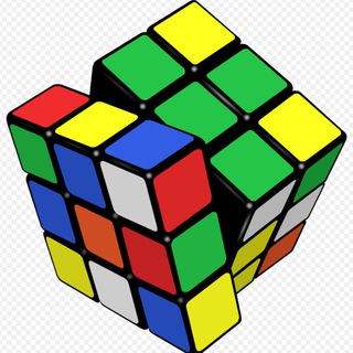
Если бы мой канал был про Oracle, MS SQL или Postgres, то его аватаркой вполне мог бы стать тот что на фото 2,
который собрать не так просто, как кажется. И если в Oracle я погружался 16 лет, то
в 2x2x2 - 2 недели, прежде чем понял что к чему.
Segreto di Pulcinella or Everything will be as you want it to be!
And why a Rubik's cube is logo for the channel ?
Why not a pyramid (as in photo 1)?
As a child, I had a pyramid and I don't remember any difficulty in it.
Or why not a mini 2x2x2?
If my channel was about Oracle, MS SQL or Postgres, then its avatar could well be the one in photo 2,
which is not as easy to assemble as it seems. And if I immersed myself in Oracle for 16 years, then in 2x2x2 - 2 weeks, before I understood what was what.
А почему собственно кубик Рубика ?
Почему не пирамидка (как на фото 1)?
В детстве у меня была пирамидка и совсем не помню какой-либо сложности в ней.
Или почему не мини 2x2x2 ?
Если бы мой канал был про Oracle, MS SQL или Postgres, то его аватаркой вполне мог бы стать тот что на фото 2,
который собрать не так просто, как кажется. И если в Oracle я погружался 16 лет, то
в 2x2x2 - 2 недели, прежде чем понял что к чему.
Segreto di Pulcinella or Everything will be as you want it to be!
And why a Rubik's cube is logo for the channel ?
Why not a pyramid (as in photo 1)?
As a child, I had a pyramid and I don't remember any difficulty in it.
Or why not a mini 2x2x2?
If my channel was about Oracle, MS SQL or Postgres, then its avatar could well be the one in photo 2,
which is not as easy to assemble as it seems. And if I immersed myself in Oracle for 16 years, then in 2x2x2 - 2 weeks, before I understood what was what.
Из курса "Теория систем" в магистратуре МИФИ мне особенно врезался в память один постулат - чем сложнее система, тем
сложнее вывести ее из равновесия или разрушить.
Кубик Рубика (3x3x3) - образцово-показательный пример сложной системы, разрушить энтропию которой,
т.е. собрать случайным образом невозможно.
Ну действительно, найти случайными поворотами 1 единственное положение из
43 252 003 274 489 856 000 может только Бог, имея бесконечный запас времени.
К слову, кубик можно собрать из любого положения за 22 хода - режим Бога -)
Я верю, что рост экспертизы в нашем ремесле происходит квантовыми скачками.
Собрать 1-ю грань кубика любой размерности очень легко, дальше начинаются игры разума.
Моим перsым открытием после тщетного ковыряния трешки было - а почему бы не взяться за мини, который я в итоге решил
после неожиданно родившейся на исходе 2й недели следующей гипотезы.
А что, если включить бритву Оккамы, отсекая лишнее: фиксируем намертво 1 кубик за начало координат( без возможности поворота),
потом решаем тот, что будет на главной диагонали и далее
выставляем остальные по диагоналям граней. В итоге осталось собрать 2 кубика, которые были дезориентированы на одном ребре.
Для их сборки, как выяснилось, существует формула сборки ( 1 из тысяч алгоритмов перестановок конкретных кубиков ), но об этом я узнал потом, когда подружил эту сладкую парочку.
Про паттерны проектирования в разработке кода я тоже узнал не сразу.
Сейчас понимаю, если бы не разборка собранного кубика в уме по определенным циклам, я бы долго возился с этой парой.
Моей следующей гипотезой стала - а не есть ли трешка по сути матрешка из мини(углы) , креста внутри ( реберные кубики ) и окошек - центральные кубики,
которые не связаны между собой.
После победы над мини, я без проблем собрал каркас (углы), решив уже известную задачу и стал интуитивно собирать ребра, как пойдет, главное, не ломая углы.
При этом я был почти уверен, что если собрать три ортогональные грани, то противоположные автоматом сложатся корректно.
Таки мне удалось собрать "половину" куба, но это был провал. Гипотеза не подтвердилась. Остальные 3 грани не сложились,
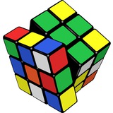
т.к. эти 3 кубика было уже не решить ( см. foto_3 ). По крайне мере, с ходу не наГуглил как ее решить.
From the course "Systems Theory" in the MEPhI master's program, one postulate especially stuck in my memory - the more complex the system, the more difficult it is to unbalance or destroy it.
The Rubik's Cube (3x3x3) is an exemplary example of a complex system, the entropy of which cannot be destroyed,
i.e., assembled randomly.
Well, indeed, only God can find 1 unique position out of
43,252,003,274,489,856,000 by random turns, having an infinite supply of time.
By the way, the cube can be assembled from any position in 22 moves - God mode -)
I believe that the growth of expertise in our craft occurs in quantum leaps.
It is very easy to assemble the 1st face of a cube of any dimension, then the mind games begin.
My first discovery after futilely picking at 3x3x3 was - why not take on the mini (2x2x2), which I eventually solved
after the following hypothesis was unexpectedly born at the end of the 2nd week.
What if we turn on Occam's razor, cutting off the excess: we fix 1 cube tightly at the origin of coordinates (without the possibility of rotation),
then we solve the one that will be on the main diagonal and then
we set the rest along the diagonals of the faces. As a result, it remained to solve 2 cubes that were disoriented on one edge.
As it turned out, there is an assembly formula for assembling them (1 of thousands of algorithms for permuting specific cubes), but I learned about this later,
when I lined up this sweet couple just right.
In my career as a developer I also did not immediately learn about design patterns in code development.
Now I understand that if it were not for disassembling the assembled cube in my mind according to certain cycles, I would have fiddled with this pair for a long time.
сложнее вывести ее из равновесия или разрушить.
Кубик Рубика (3x3x3) - образцово-показательный пример сложной системы, разрушить энтропию которой,
т.е. собрать случайным образом невозможно.
Ну действительно, найти случайными поворотами 1 единственное положение из
43 252 003 274 489 856 000 может только Бог, имея бесконечный запас времени.
К слову, кубик можно собрать из любого положения за 22 хода - режим Бога -)
Я верю, что рост экспертизы в нашем ремесле происходит квантовыми скачками.
Собрать 1-ю грань кубика любой размерности очень легко, дальше начинаются игры разума.
Моим перsым открытием после тщетного ковыряния трешки было - а почему бы не взяться за мини, который я в итоге решил
после неожиданно родившейся на исходе 2й недели следующей гипотезы.
А что, если включить бритву Оккамы, отсекая лишнее: фиксируем намертво 1 кубик за начало координат( без возможности поворота),
потом решаем тот, что будет на главной диагонали и далее
выставляем остальные по диагоналям граней. В итоге осталось собрать 2 кубика, которые были дезориентированы на одном ребре.
Для их сборки, как выяснилось, существует формула сборки ( 1 из тысяч алгоритмов перестановок конкретных кубиков ), но об этом я узнал потом, когда подружил эту сладкую парочку.
Про паттерны проектирования в разработке кода я тоже узнал не сразу.
Сейчас понимаю, если бы не разборка собранного кубика в уме по определенным циклам, я бы долго возился с этой парой.
Моей следующей гипотезой стала - а не есть ли трешка по сути матрешка из мини(углы) , креста внутри ( реберные кубики ) и окошек - центральные кубики,
которые не связаны между собой.
После победы над мини, я без проблем собрал каркас (углы), решив уже известную задачу и стал интуитивно собирать ребра, как пойдет, главное, не ломая углы.
При этом я был почти уверен, что если собрать три ортогональные грани, то противоположные автоматом сложатся корректно.
Таки мне удалось собрать "половину" куба, но это был провал. Гипотеза не подтвердилась. Остальные 3 грани не сложились,
т.к. эти 3 кубика было уже не решить ( см. foto_3 ). По крайне мере, с ходу не наГуглил как ее решить.
From the course "Systems Theory" in the MEPhI master's program, one postulate especially stuck in my memory - the more complex the system, the more difficult it is to unbalance or destroy it.
The Rubik's Cube (3x3x3) is an exemplary example of a complex system, the entropy of which cannot be destroyed,
i.e., assembled randomly.
Well, indeed, only God can find 1 unique position out of
43,252,003,274,489,856,000 by random turns, having an infinite supply of time.
By the way, the cube can be assembled from any position in 22 moves - God mode -)
I believe that the growth of expertise in our craft occurs in quantum leaps.
It is very easy to assemble the 1st face of a cube of any dimension, then the mind games begin.
My first discovery after futilely picking at 3x3x3 was - why not take on the mini (2x2x2), which I eventually solved
after the following hypothesis was unexpectedly born at the end of the 2nd week.
What if we turn on Occam's razor, cutting off the excess: we fix 1 cube tightly at the origin of coordinates (without the possibility of rotation),
then we solve the one that will be on the main diagonal and then
we set the rest along the diagonals of the faces. As a result, it remained to solve 2 cubes that were disoriented on one edge.
As it turned out, there is an assembly formula for assembling them (1 of thousands of algorithms for permuting specific cubes), but I learned about this later,
when I lined up this sweet couple just right.
In my career as a developer I also did not immediately learn about design patterns in code development.
Now I understand that if it were not for disassembling the assembled cube in my mind according to certain cycles, I would have fiddled with this pair for a long time.
Аналогично, в Greenplum разработчик задает корректные ключи распределения таблиц без перекосов и думает, что пора выкатываться в пром, но реальность сложнее
и начинает проявляться уже при join-е 3х таблиц по несогласованным с их хэшами ключам, если одна таблица-блудница
должна сопрягаться с всякими другими по требованиям бизнеса по разным ключам в разных запросах или в одном и том же.
Или другой весьма поучительный пример потенциальной бомбы на тему foto_3, когда мы грузим ключи банковских проводок в хаб Data-Vault.
Мы блестяще построили защиту от дублирования старых, уже загруженных ранее документов, но увы забыли, что когда объем хаба вырастет вдвое,
то и время поиска старых документов в хабе вырастет вдвое.
А почему ? Потому что ситом для просеивания проводок является весь хаб целиком, а не множество, размер которого можно контролировать, например кодом источника и датой проводки.
Решение в итоге не масштабируется - кубик не собран.
Вернемся к нашим баранам. В итоге, моя гипотеза матрешек кубика была состоятельна,
но мне пришлось воспользоваться подсказкой, что после каркаса надо собирать строго определенные
слои, точнее крайние, что расходится с традиционной системой послойной сборки, где углы, однако, не фиксируются.
И вот наконец, остался средний слой и собран кубик ... но снова грабли - вылетели те самые центральные окошки.
Я сломал ребра и стал собирать снова, но чтобы окошки не гуляли и в итоге пришел к конфигурации
с двумя нерешенными кубиками ( как на foto_4 ), на разворот которых требуется 12 ходов, на что тоже есть своя формула,
половину которой я подсмотрел.
Тут как видим, здание было не собрано даже на половину, исходя из того, что максимальная трудоемкость решения любой конфигурации - 22 хода,
а мне до цели осталось 12.
В итоге - успех, но какой ценой. Энтропия как мера хаоса любой информационной системы - это тот же кубик,
которую можно обуздать, если знать стратегию, которая упрощает решение проблемы шаг за шагом -
углы ( проблема решена на кубике меньшей размерности ) => ребра двух крайних граней => срединный слой, в котором
все конфигурации зверушки изучены и описаны формулами.
Известно, что на ошибки проектирования тратится 90% бюджета проекта.
Если, я донес хотя бы до 1 человека, как важно определиться с концепцией вашего здания DWH и знать типовые шаблоны проектирования кода,
которые тут иногда публикуются, буду считать, что этот лонгрид был не зря.
Similarly, in Greenplum, the developer sets the correct table distribution keys without skew and thinks that it's time to roll out to production, but the reality is more complicated
and begins to manifest itself already when joining 3 tables by keys that are not consistent with their hashes, if one harlot table
must be matched with many others according to business requirements by different keys in different queries or in the same one.
Or another very instructive example of a potential bomb on the topic of foto_3, when we load bank transaction keys into the Data-Vault hub.
We brilliantly built protection against duplication of old, previously loaded documents, but alas, we forgot that when the hub volume doubles,
then the time to search for old documents in the hub will also double.
And why? Because the sieve for sifting transactions is the entire hub as a whole, and not a set, the size of which can be controlled, for example, by the source code and transaction date.
The solution ultimately does not scale - the cube is not assembled.
Let's get back to our sheep. Ultimately, my hypothesis of the cube's nesting dolls was consistent,
but I had to use the hint that after the frame, strictly defined
layers must be assembled, or rather the outer ones, which diverges from the traditional layer-by-layer assembly system, where the corners, however, are not fixed.
And finally, the middle layer remained and the cube was assembled ... but again a rake - those very central windows flew out.
👏3