
Data Science Machine Learning Data Analysis
Photo
## 🔹 Best Practices for CNN Development
1. Start with pretrained models when possible
2. Use progressive resizing (start with small images, then increase)
3. Monitor class activation maps to debug model focus areas
4. Apply test-time augmentation (TTA) for better inference
5. Use label smoothing for classification tasks
6. Implement learning rate warmup for large batch training
---
### 📌 What's Next?
In Part 4, we'll cover:
➡️ Recurrent Neural Networks (RNNs/LSTMs)
➡️ Sequence Modeling
➡️ Attention Mechanisms
➡️ Transformer Architectures
#PyTorch #DeepLearning #ComputerVision 🚀
Practice Exercises:
1. Modify the CNN to use depthwise separable convolutions
2. Implement a ResNet-18 from scratch
3. Apply Grad-CAM to visualize model decisions
4. Train on CIFAR-100 with CutMix augmentation
5. Compare Adam vs. SGD with momentum performance
https://t.iss.one/DataScienceM🌟
1. Start with pretrained models when possible
2. Use progressive resizing (start with small images, then increase)
3. Monitor class activation maps to debug model focus areas
4. Apply test-time augmentation (TTA) for better inference
5. Use label smoothing for classification tasks
6. Implement learning rate warmup for large batch training
# Label smoothing example
criterion = nn.CrossEntropyLoss(label_smoothing=0.1)

# Learning rate warmup
def warmup_lr(epoch, warmup_epochs=5, base_lr=0.001):
    return base_lr * (epoch + 1) / warmup_epochs if epoch < warmup_epochs else base_lr
---
### 📌 What's Next?
In Part 4, we'll cover:
➡️ Recurrent Neural Networks (RNNs/LSTMs)
➡️ Sequence Modeling
➡️ Attention Mechanisms
➡️ Transformer Architectures
#PyTorch #DeepLearning #ComputerVision 🚀
Practice Exercises:
1. Modify the CNN to use depthwise separable convolutions
2. Implement a ResNet-18 from scratch
3. Apply Grad-CAM to visualize model decisions
4. Train on CIFAR-100 with CutMix augmentation
5. Compare Adam vs. SGD with momentum performance
# Depthwise separable convolution example
class DepthwiseSeparableConv(nn.Module):
    def __init__(self, in_channels, out_channels, stride=1):
        super().__init__()
        self.depthwise = nn.Conv2d(in_channels, in_channels, kernel_size=3,
                                  stride=stride, padding=1, groups=in_channels)
        self.pointwise = nn.Conv2d(in_channels, out_channels, kernel_size=1)

    def forward(self, x):
        return self.pointwise(self.depthwise(x))
https://t.iss.one/DataScienceM
Please open Telegram to view this post
VIEW IN TELEGRAM
Telegram
Data Science Machine Learning Data Analysis
This channel is for Programmers, Coders, Software Engineers.
1- Data Science
2- Machine Learning
3- Data Visualization
4- Artificial Intelligence
5- Data Analysis
6- Statistics
7- Deep Learning
Cross promotion and ads: @hussein_sheikho
1- Data Science
2- Machine Learning
3- Data Visualization
4- Artificial Intelligence
5- Data Analysis
6- Statistics
7- Deep Learning
Cross promotion and ads: @hussein_sheikho
❤1
Data Science Machine Learning Data Analysis
Photo
# 📚 PyTorch Tutorial for Beginners - Part 4/6: Sequence Modeling with RNNs, LSTMs & Attention
#PyTorch #DeepLearning #NLP #RNN #LSTM #Transformer
Welcome to Part 4 of our PyTorch series! This comprehensive lesson dives deep into sequence modeling, covering recurrent networks, attention mechanisms, and transformer architectures with practical implementations.
---
## 🔹 Introduction to Sequence Modeling
### Key Challenges with Sequences
1. Variable Length: Sequences can be arbitrarily long (sentences, time series)
2. Temporal Dependencies: Current output depends on previous inputs
3. Context Preservation: Need to maintain long-range relationships
### Comparison of Approaches
| Model Type | Pros | Cons | Typical Use Cases |
|------------------|---------------------------------------|---------------------------------------|---------------------------------|
| RNN | Simple, handles sequences | Struggles with long-term dependencies | Short time series, char-level NLP |
| LSTM | Better long-term memory | Computationally heavier | Machine translation, speech recognition |
| GRU | LSTM-like with fewer parameters | Still limited context | Medium-length sequences |
| Transformer | Parallel processing, global context | Memory intensive for long sequences | Modern NLP, any sequence task |
---
## 🔹 Recurrent Neural Networks (RNNs)
### 1. Basic RNN Architecture
### 2. The Vanishing Gradient Problem
RNNs struggle with long sequences due to:
- Repeated multiplication of small gradients through time
- Exponential decay of gradient information
Solutions:
- Gradient clipping
- Architectural changes (LSTM, GRU)
- Skip connections
---
## 🔹 Long Short-Term Memory (LSTM) Networks
### 1. LSTM Core Concepts

Key Components:
- Forget Gate: Decides what information to discard
- Input Gate: Updates cell state with new information
- Output Gate: Determines next hidden state
### 2. PyTorch Implementation
#PyTorch #DeepLearning #NLP #RNN #LSTM #Transformer
Welcome to Part 4 of our PyTorch series! This comprehensive lesson dives deep into sequence modeling, covering recurrent networks, attention mechanisms, and transformer architectures with practical implementations.
---
## 🔹 Introduction to Sequence Modeling
### Key Challenges with Sequences
1. Variable Length: Sequences can be arbitrarily long (sentences, time series)
2. Temporal Dependencies: Current output depends on previous inputs
3. Context Preservation: Need to maintain long-range relationships
### Comparison of Approaches
| Model Type | Pros | Cons | Typical Use Cases |
|------------------|---------------------------------------|---------------------------------------|---------------------------------|
| RNN | Simple, handles sequences | Struggles with long-term dependencies | Short time series, char-level NLP |
| LSTM | Better long-term memory | Computationally heavier | Machine translation, speech recognition |
| GRU | LSTM-like with fewer parameters | Still limited context | Medium-length sequences |
| Transformer | Parallel processing, global context | Memory intensive for long sequences | Modern NLP, any sequence task |
---
## 🔹 Recurrent Neural Networks (RNNs)
### 1. Basic RNN Architecture
class VanillaRNN(nn.Module):
    def __init__(self, input_size, hidden_size, output_size):
        super().__init__()
        self.hidden_size = hidden_size
        self.rnn = nn.RNN(input_size, hidden_size, batch_first=True)
        self.fc = nn.Linear(hidden_size, output_size)

    def forward(self, x, hidden=None):
        # x shape: (batch, seq_len, input_size)
        out, hidden = self.rnn(x, hidden)
        # Only use last output for classification
        out = self.fc(out[:, -1, :])
        return out

# Usage
rnn = VanillaRNN(input_size=10, hidden_size=20, output_size=5)
x = torch.randn(3, 15, 10)  # (batch=3, seq_len=15, input_size=10)
output = rnn(x)
### 2. The Vanishing Gradient Problem
RNNs struggle with long sequences due to:
- Repeated multiplication of small gradients through time
- Exponential decay of gradient information
Solutions:
- Gradient clipping
- Architectural changes (LSTM, GRU)
- Skip connections
---
## 🔹 Long Short-Term Memory (LSTM) Networks
### 1. LSTM Core Concepts

Key Components:
- Forget Gate: Decides what information to discard
- Input Gate: Updates cell state with new information
- Output Gate: Determines next hidden state
### 2. PyTorch Implementation
class LSTMModel(nn.Module):
    def __init__(self, input_size, hidden_size, num_layers, output_size):
        super().__init__()
        self.lstm = nn.LSTM(input_size, hidden_size, num_layers,
                           batch_first=True, dropout=0.2 if num_layers>1 else 0)
        self.fc = nn.Linear(hidden_size, output_size)

    def forward(self, x):
        # Initialize hidden state and cell state
        h0 = torch.zeros(self.lstm.num_layers, x.size(0),
                        self.lstm.hidden_size).to(x.device)
        c0 = torch.zeros_like(h0)

        out, (hn, cn) = self.lstm(x, (h0, c0))
        out = self.fc(out[:, -1, :])
        return out

# Bidirectional LSTM example
bidir_lstm = nn.LSTM(input_size=10, hidden_size=20, num_layers=2,
                    bidirectional=True, batch_first=True)
Data Science Machine Learning Data Analysis
Photo
### 3. Practical Tips for LSTMs
- Initialization: Orthogonal initialization for recurrent weights
- Dropout: Use
- Sequence Packing: For variable-length sequences:
---
## 🔹 Gated Recurrent Units (GRUs)
### Simplified Alternative to LSTM
GRU vs LSTM:
- GRU combines forget and input gates into update gate
- GRU merges cell state and hidden state
- Typically faster to train with comparable performance
---
## 🔹 Attention Mechanisms
### 1. Why Attention?
- Addresses information bottleneck in encoder-decoder architectures
- Allows dynamic focus on relevant parts of input
- Enables interpretability (visualize attention weights)
### 2. Basic Attention Implementation
### 3. Visualizing Attention
---
## 🔹 Transformer Architectures
### 1. Core Components
Key Innovations:
- Self-Attention: Captures relationships between all sequence positions
- Positional Encoding: Injects sequence order information
- Layer Normalization: Stabilizes training
- Feed-Forward Networks: Applied position-wise
- Initialization: Orthogonal initialization for recurrent weights
- Dropout: Use
dropout between LSTM layers (not on last layer)- Sequence Packing: For variable-length sequences:
from torch.nn.utils.rnn import pack_padded_sequence, pad_packed_sequence

# Assume 'lengths' contains original sequence lengths
packed_input = pack_padded_sequence(x, lengths, batch_first=True, enforce_sorted=False)
packed_output, (hn, cn) = lstm(packed_input)
output, _ = pad_packed_sequence(packed_output, batch_first=True)
---
## 🔹 Gated Recurrent Units (GRUs)
### Simplified Alternative to LSTM
class GRUModel(nn.Module):
    def __init__(self, input_size, hidden_size, num_layers, output_size):
        super().__init__()
        self.gru = nn.GRU(input_size, hidden_size, num_layers,
                         batch_first=True, dropout=0.2)
        self.fc = nn.Linear(hidden_size, output_size)

    def forward(self, x):
        out, hn = self.gru(x)
        out = self.fc(out[:, -1, :])
        return out
GRU vs LSTM:
- GRU combines forget and input gates into update gate
- GRU merges cell state and hidden state
- Typically faster to train with comparable performance
---
## 🔹 Attention Mechanisms
### 1. Why Attention?
- Addresses information bottleneck in encoder-decoder architectures
- Allows dynamic focus on relevant parts of input
- Enables interpretability (visualize attention weights)
### 2. Basic Attention Implementation
class Attention(nn.Module):
    def __init__(self, hidden_size):
        super().__init__()
        self.attention = nn.Linear(hidden_size, hidden_size)
        self.context = nn.Parameter(torch.randn(hidden_size))

    def forward(self, hidden_states):
        # hidden_states shape: (batch, seq_len, hidden_size)

        # Compute attention scores
        energies = torch.tanh(self.attention(hidden_states))
        scores = torch.matmul(energies, self.context)
        alphas = torch.softmax(scores, dim=1)

        # Compute context vector
        context = torch.sum(hidden_states * alphas.unsqueeze(-1), dim=1)
        return context, alphas

# Integrated with RNN
class AttnRNN(nn.Module):
    def __init__(self, input_size, hidden_size, output_size):
        super().__init__()
        self.rnn = nn.GRU(input_size, hidden_size, batch_first=True)
        self.attention = Attention(hidden_size)
        self.fc = nn.Linear(hidden_size, output_size)

    def forward(self, x):
        out, _ = self.rnn(x)
        context, alphas = self.attention(out)
        return self.fc(context), alphas
### 3. Visualizing Attention
def plot_attention(input_text, alphas):
    fig, ax = plt.subplots(figsize=(12, 4))
    ax.imshow(alphas.cpu().numpy(), cmap='viridis')
    ax.set_xticks(range(len(input_text.split())))
    ax.set_xticklabels(input_text.split(), rotation=45)
    ax.set_yticks([0])
    ax.set_yticklabels(['Attention'])
    plt.tight_layout()
    plt.show()
---
## 🔹 Transformer Architectures
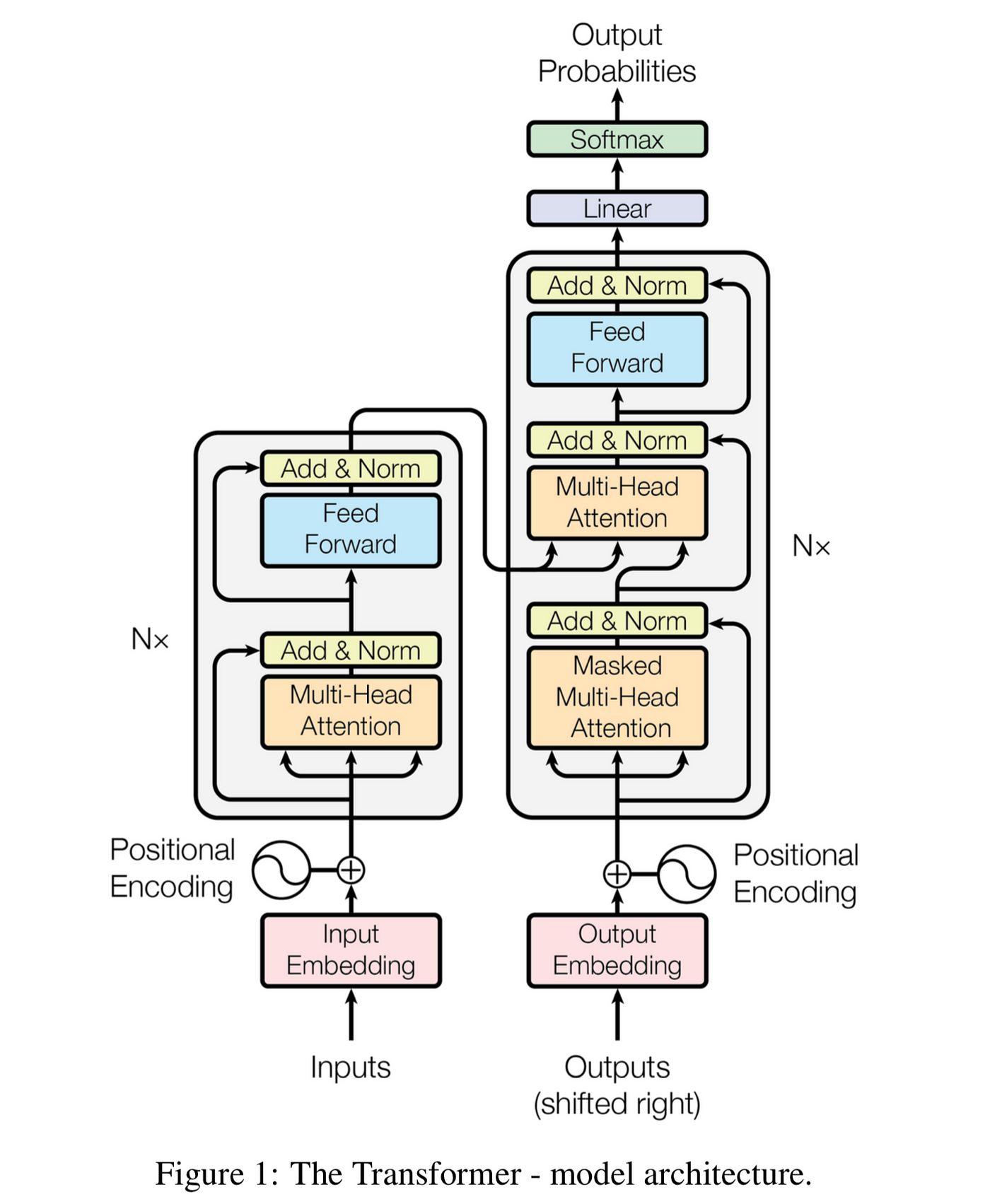
### 1. Core Components

Key Innovations:
- Self-Attention: Captures relationships between all sequence positions
- Positional Encoding: Injects sequence order information
- Layer Normalization: Stabilizes training
- Feed-Forward Networks: Applied position-wise
❤1
Data Science Machine Learning Data Analysis
Photo
### 2. Implementing Multi-Head Attention
### **3. Complete Transformer Block**
### 4. Positional Encoding
---
class MultiHeadAttention(nn.Module):
    def __init__(self, embed_size, heads):
        super().__init__()
        self.embed_size = embed_size
        self.heads = heads
        self.head_dim = embed_size // heads

        assert self.head_dim * heads == embed_size, "Embed size needs to be divisible by heads"

        self.values = nn.Linear(self.head_dim, self.head_dim, bias=False)
        self.keys = nn.Linear(self.head_dim, self.head_dim, bias=False)
        self.queries = nn.Linear(self.head_dim, self.head_dim, bias=False)
        self.fc_out = nn.Linear(heads * self.head_dim, embed_size)

    def forward(self, values, keys, query, mask=None):
        N = query.shape[0]
        value_len, key_len, query_len = values.shape[1], keys.shape[1], query.shape[1]

        # Split embedding into self.heads pieces
        values = values.reshape(N, value_len, self.heads, self.head_dim)
        keys = keys.reshape(N, key_len, self.heads, self.head_dim)
        queries = query.reshape(N, query_len, self.heads, self.head_dim)

        # Attention scores
        energy = torch.einsum("nqhd,nkhd->nhqk", [queries, keys])

        if mask is not None:
            energy = energy.masked_fill(mask == 0, float("-1e20"))

        attention = torch.softmax(energy / (self.embed_size ** (1/2)), dim=3)

        out = torch.einsum("nhql,nlhd->nqhd", [attention, values]).reshape(
            N, query_len, self.heads * self.head_dim
        )

        out = self.fc_out(out)
        return out
### **3. Complete Transformer Block**
class TransformerBlock(nn.Module):
    def __init__(self, embed_size, heads, dropout, forward_expansion):
        super().__init__()
        self.attention = MultiHeadAttention(embed_size, heads)
        self.norm1 = nn.LayerNorm(embed_size)
        self.norm2 = nn.LayerNorm(embed_size)

        self.feed_forward = nn.Sequential(
            nn.Linear(embed_size, forward_expansion * embed_size),
            nn.ReLU(),
            nn.Linear(forward_expansion * embed_size, embed_size)
        )

        self.dropout = nn.Dropout(dropout)

    def forward(self, value, key, query, mask):
        attention = self.attention(value, key, query, mask)
        x = self.dropout(self.norm1(attention + query))
        forward = self.feed_forward(x)
        out = self.dropout(self.norm2(forward + x))
        return out
### 4. Positional Encoding
class PositionalEncoding(nn.Module):
    def __init__(self, embed_size, max_len=100):
        super().__init__()
        pe = torch.zeros(max_len, embed_size)
        position = torch.arange(0, max_len, dtype=torch.float).unsqueeze(1)
        div_term = torch.exp(torch.arange(0, embed_size, 2).float() * (-math.log(10000.0) / embed_size)

        pe[:, 0::2] = torch.sin(position * div_term)
        pe[:, 1::2] = torch.cos(position * div_term)
        pe = pe.unsqueeze(0)
        self.register_buffer('pe', pe)

    def forward(self, x):
        return x + self.pe[:, :x.size(1)]
---
Data Science Machine Learning Data Analysis
Photo
## 🔹 Practical Sequence Modeling Tasks
### 1. Text Classification Pipeline
### 2. Sequence-to-Sequence (Seq2Seq) Model
---
## 🔹 Best Practices for Sequence Modeling
1. Always use packed sequences for variable-length inputs
2. Gradient clipping is essential for RNNs/LSTMs (1-5 norm)
3. Teacher forcing helps seq2seq models converge faster
4. Bidirectional RNNs significantly improve performance
5. Layer normalization stabilizes transformer training
6. Warmup learning rate for transformer models
### 1. Text Classification Pipeline
from torchtext.legacy import data

# Define fields
TEXT = data.Field(tokenize='spacy', lower=True, include_lengths=True)
LABEL = data.LabelField(dtype=torch.float)

# Load dataset (e.g., IMDB)
train_data, test_data = datasets.IMDB.splits(TEXT, LABEL)

# Build vocabulary
TEXT.build_vocab(train_data, max_size=25000,
                vectors="glove.6B.100d", unk_init=torch.Tensor.normal_)
LABEL.build_vocab(train_data)

# Create iterators
train_loader, test_loader = data.BucketIterator.splits(
    (train_data, test_data),
    batch_size=64,
    sort_within_batch=True,
    sort_key=lambda x: len(x.text),
    device=device
)

# Model definition
class TextClassifier(nn.Module):
    def __init__(self, vocab_size, embed_dim, hidden_dim, output_dim, n_layers):
        super().__init__()
        self.embedding = nn.Embedding(vocab_size, embed_dim)
        self.rnn = nn.LSTM(embed_dim, hidden_dim, n_layers,
                          bidirectional=True, dropout=0.5)
        self.fc = nn.Linear(hidden_dim * 2, output_dim)
        self.dropout = nn.Dropout(0.5)

    def forward(self, text, text_lengths):
        embedded = self.dropout(self.embedding(text))
        packed_embedded = nn.utils.rnn.pack_padded_sequence(
            embedded, text_lengths.cpu(), batch_first=False, enforce_sorted=False
        )
        packed_output, (hidden, cell) = self.rnn(packed_embedded)
        hidden = self.dropout(torch.cat((hidden[-2,:,:], hidden[-1,:,:]), dim=1))
        return self.fc(hidden)
### 2. Sequence-to-Sequence (Seq2Seq) Model
class Encoder(nn.Module):
    def __init__(self, input_dim, emb_dim, hidden_dim, n_layers, dropout):
        super().__init__()
        self.embedding = nn.Embedding(input_dim, emb_dim)
        self.rnn = nn.LSTM(emb_dim, hidden_dim, n_layers, dropout=dropout)
        self.dropout = nn.Dropout(dropout)

    def forward(self, src):
        embedded = self.dropout(self.embedding(src))
        outputs, (hidden, cell) = self.rnn(embedded)
        return hidden, cell

class Decoder(nn.Module):
    def __init__(self, output_dim, emb_dim, hidden_dim, n_layers, dropout):
        super().__init__()
        self.embedding = nn.Embedding(output_dim, emb_dim)
        self.rnn = nn.LSTM(emb_dim, hidden_dim, n_layers, dropout=dropout)
        self.fc = nn.Linear(hidden_dim, output_dim)
        self.dropout = nn.Dropout(dropout)

    def forward(self, input, hidden, cell):
        input = input.unsqueeze(0)
        embedded = self.dropout(self.embedding(input))
        output, (hidden, cell) = self.rnn(embedded, (hidden, cell))
        prediction = self.fc(output.squeeze(0))
        return prediction, hidden, cell

class Seq2Seq(nn.Module):
    def __init__(self, encoder, decoder, device):
        super().__init__()
        self.encoder = encoder
        self.decoder = decoder
        self.device = device

    def forward(self, src, trg, teacher_forcing_ratio=0.5):
        trg_len = trg.shape[0]
        batch_size = trg.shape[1]
        trg_vocab_size = self.decoder.fc.out_features

        outputs = torch.zeros(trg_len, batch_size, trg_vocab_size).to(self.device)
        hidden, cell = self.encoder(src)

        input = trg[0,:]

        for t in range(1, trg_len):
            output, hidden, cell = self.decoder(input, hidden, cell)
            outputs[t] = output
            teacher_force = random.random() < teacher_forcing_ratio
            top1 = output.argmax(1)
            input = trg[t] if teacher_force else top1

        return outputs
---
## 🔹 Best Practices for Sequence Modeling
1. Always use packed sequences for variable-length inputs
2. Gradient clipping is essential for RNNs/LSTMs (1-5 norm)
3. Teacher forcing helps seq2seq models converge faster
4. Bidirectional RNNs significantly improve performance
5. Layer normalization stabilizes transformer training
6. Warmup learning rate for transformer models
❤1
Data Science Machine Learning Data Analysis
Photo
# Learning rate scheduler for transformers
def lr_schedule(step, d_model=512, warmup_steps=4000):
    arg1 = step ** -0.5
    arg2 = step * (warmup_steps ** -1.5)
    return (d_model ** -0.5) * min(step ** -0.5, step * warmup_steps ** -1.5)
---
### **📌 What's Next?
In **Part 5, we'll cover:
➡️ Generative Models (GANs, VAEs)
➡️ Reinforcement Learning with PyTorch
➡️ Model Optimization & Deployment
➡️ PyTorch Lightning Best Practices
#PyTorch #DeepLearning #NLP #Transformers 🚀
Practice Exercises:
1. Implement a character-level language model with LSTM
2. Add attention visualization to a sentiment analysis model
3. Build a transformer from scratch for machine translation
4. Compare teacher forcing ratios in seq2seq training
5. Implement beam search for decoder inference
# Character-level LSTM starter
class CharLSTM(nn.Module):
    def __init__(self, vocab_size, hidden_size, n_layers):
        super().__init__()
        self.embed = nn.Embedding(vocab_size, hidden_size)
        self.lstm = nn.LSTM(hidden_size, hidden_size, n_layers, batch_first=True)
        self.fc = nn.Linear(hidden_size, vocab_size)

    def forward(self, x, hidden=None):
        x = self.embed(x)
        out, hidden = self.lstm(x, hidden)
        return self.fc(out), hidden
🔥2❤1
Data Science Machine Learning Data Analysis
Photo
# 📚 PyTorch Tutorial for Beginners - Part 5/6: Generative Models & Advanced Topics
#PyTorch #DeepLearning #GANs #VAEs #ReinforcementLearning #Deployment
Welcome to Part 5 of our PyTorch series! This comprehensive lesson explores generative modeling, reinforcement learning, model optimization, and deployment strategies with practical implementations.
---
## 🔹 Generative Adversarial Networks (GANs)
### 1. GAN Core Concepts

Key Components:
- Generator: Creates fake samples from noise (typically a transposed CNN)
- Discriminator: Distinguishes real vs. fake samples (CNN classifier)
- Adversarial Training: The two networks compete in a minimax game
### 2. DCGAN Implementation
### 3. GAN Training Loop
#PyTorch #DeepLearning #GANs #VAEs #ReinforcementLearning #Deployment
Welcome to Part 5 of our PyTorch series! This comprehensive lesson explores generative modeling, reinforcement learning, model optimization, and deployment strategies with practical implementations.
---
## 🔹 Generative Adversarial Networks (GANs)
### 1. GAN Core Concepts

Key Components:
- Generator: Creates fake samples from noise (typically a transposed CNN)
- Discriminator: Distinguishes real vs. fake samples (CNN classifier)
- Adversarial Training: The two networks compete in a minimax game
### 2. DCGAN Implementation
class Generator(nn.Module):
    def __init__(self, latent_dim, img_channels, features_g):
        super().__init__()
        self.net = nn.Sequential(
            # Input: N x latent_dim x 1 x 1
            nn.ConvTranspose2d(latent_dim, features_g*8, 4, 1, 0, bias=False),
            nn.BatchNorm2d(features_g*8),
            nn.ReLU(),
            # 4x4
            nn.ConvTranspose2d(features_g*8, features_g*4, 4, 2, 1, bias=False),
            nn.BatchNorm2d(features_g*4),
            nn.ReLU(),
            # 8x8
            nn.ConvTranspose2d(features_g*4, features_g*2, 4, 2, 1, bias=False),
            nn.BatchNorm2d(features_g*2),
            nn.ReLU(),
            # 16x16
            nn.ConvTranspose2d(features_g*2, img_channels, 4, 2, 1, bias=False),
            nn.Tanh()
            # 32x32
        )

    def forward(self, x):
        return self.net(x)

class Discriminator(nn.Module):
    def __init__(self, img_channels, features_d):
        super().__init__()
        self.net = nn.Sequential(
            # Input: N x img_channels x 32 x 32
            nn.Conv2d(img_channels, features_d, 4, 2, 1, bias=False),
            nn.LeakyReLU(0.2),
            # 16x16
            nn.Conv2d(features_d, features_d*2, 4, 2, 1, bias=False),
            nn.BatchNorm2d(features_d*2),
            nn.LeakyReLU(0.2),
            # 8x8
            nn.Conv2d(features_d*2, features_d*4, 4, 2, 1, bias=False),
            nn.BatchNorm2d(features_d*4),
            nn.LeakyReLU(0.2),
            # 4x4
            nn.Conv2d(features_d*4, 1, 4, 1, 0, bias=False),
            nn.Sigmoid()
        )

    def forward(self, x):
        return self.net(x)

# Initialize
gen = Generator(latent_dim=100, img_channels=3, features_g=64).to(device)
disc = Discriminator(img_channels=3, features_d=64).to(device)

# Loss and optimizers
criterion = nn.BCELoss()
opt_gen = optim.Adam(gen.parameters(), lr=0.0002, betas=(0.5, 0.999))
opt_disc = optim.Adam(disc.parameters(), lr=0.0002, betas=(0.5, 0.999))
### 3. GAN Training Loop
def train_gan(gen, disc, loader, num_epochs):
    fixed_noise = torch.randn(32, 100, 1, 1).to(device)

    for epoch in range(num_epochs):
        for batch_idx, (real, _) in enumerate(loader):
            real = real.to(device)
            noise = torch.randn(real.size(0), 100, 1, 1).to(device)
            fake = gen(noise)

            # Train Discriminator
            disc_real = disc(real).view(-1)
            loss_disc_real = criterion(disc_real, torch.ones_like(disc_real))
            disc_fake = disc(fake.detach()).view(-1)
            loss_disc_fake = criterion(disc_fake, torch.zeros_like(disc_fake))
            loss_disc = (loss_disc_real + loss_disc_fake) / 2
            disc.zero_grad()
            loss_disc.backward()
            opt_disc.step()

            # Train Generator
            output = disc(fake).view(-1)
            loss_gen = criterion(output, torch.ones_like(output))
            gen.zero_grad()
            loss_gen.backward()
            opt_gen.step()

        # Visualization
        with torch.no_grad():
            fake = gen(fixed_noise)
            save_image(fake, f"gan_samples/epoch_{epoch}.png", normalize=True)
❤1
Data Science Machine Learning Data Analysis
Photo
### 4. GAN Training Challenges & Solutions
| Problem | Solution | Implementation Tips |
|-----------------------|-----------------------------------|---------------------------------------|
| Mode Collapse | Mini-batch discrimination | Use
| Vanishing Gradients | Wasserstein GAN with GP | Clip critic weights or use gradient penalty |
| Unstable Training | Two Time-Scale Update Rule (TTUR) | Different learning rates for G/D |
| Poor Image Quality | Spectral Normalization |
---
## 🔹 Variational Autoencoders (VAEs)
### 1. VAE Core Concepts

Key Components:
- Encoder: Maps input to latent space distribution parameters (μ, σ)
- Reparameterization Trick: Allows backpropagation through sampling
- Decoder: Reconstructs input from latent samples
### 2. VAE Implementation
### 3. Conditional VAE (CVAE)
---
| Problem | Solution | Implementation Tips |
|-----------------------|-----------------------------------|---------------------------------------|
| Mode Collapse | Mini-batch discrimination | Use
torch.cat for batch statistics || Vanishing Gradients | Wasserstein GAN with GP | Clip critic weights or use gradient penalty |
| Unstable Training | Two Time-Scale Update Rule (TTUR) | Different learning rates for G/D |
| Poor Image Quality | Spectral Normalization |
torch.nn.utils.spectral_norm layers |---
## 🔹 Variational Autoencoders (VAEs)
### 1. VAE Core Concepts

Key Components:
- Encoder: Maps input to latent space distribution parameters (μ, σ)
- Reparameterization Trick: Allows backpropagation through sampling
- Decoder: Reconstructs input from latent samples
### 2. VAE Implementation
class VAE(nn.Module):
    def __init__(self, input_dim, hidden_dim, latent_dim):
        super().__init__()

        # Encoder
        self.encoder = nn.Sequential(
            nn.Linear(input_dim, hidden_dim),
            nn.ReLU(),
            nn.Linear(hidden_dim, hidden_dim),
            nn.ReLU()
        )

        # Latent space parameters
        self.fc_mu = nn.Linear(hidden_dim, latent_dim)
        self.fc_var = nn.Linear(hidden_dim, latent_dim)

        # Decoder
        self.decoder = nn.Sequential(
            nn.Linear(latent_dim, hidden_dim),
            nn.ReLU(),
            nn.Linear(hidden_dim, hidden_dim),
            nn.ReLU(),
            nn.Linear(hidden_dim, input_dim),
            nn.Sigmoid()
        )

    def encode(self, x):
        h = self.encoder(x)
        return self.fc_mu(h), self.fc_var(h)

    def reparameterize(self, mu, logvar):
        std = torch.exp(0.5 * logvar)
        eps = torch.randn_like(std)
        return mu + eps * std

    def decode(self, z):
        return self.decoder(z)

    def forward(self, x):
        mu, logvar = self.encode(x)
        z = self.reparameterize(mu, logvar)
        return self.decode(z), mu, logvar

# Loss function
def vae_loss(recon_x, x, mu, logvar):
    BCE = nn.functional.binary_cross_entropy(recon_x, x, reduction='sum')
    KLD = -0.5 * torch.sum(1 + logvar - mu.pow(2) - logvar.exp())
    return BCE + KLD
### 3. Conditional VAE (CVAE)
class CVAE(nn.Module):
    def __init__(self, input_dim, hidden_dim, latent_dim, num_classes):
        super().__init__()
        self.label_emb = nn.Embedding(num_classes, num_classes)

        # Encoder now takes both image and label
        self.encoder = nn.Sequential(
            nn.Linear(input_dim + num_classes, hidden_dim),
            nn.ReLU()
        )

        # Rest remains similar to VAE...
---
Data Science Machine Learning Data Analysis
Photo
## 🔹 Reinforcement Learning with PyTorch
### 1. Deep Q-Network (DQN)
### 2. Policy Gradient Methods
---
## 🔹 Model Optimization & Deployment
### 1. Quantization
### 1. Deep Q-Network (DQN)
class DQN(nn.Module):
    def __init__(self, input_dim, output_dim):
        super().__init__()
        self.fc = nn.Sequential(
            nn.Linear(input_dim, 128),
            nn.ReLU(),
            nn.Linear(128, 128),
            nn.ReLU(),
            nn.Linear(128, output_dim)
        )

    def forward(self, x):
        return self.fc(x)

# Experience Replay
class ReplayBuffer:
    def __init__(self, capacity):
        self.buffer = deque(maxlen=capacity)

    def push(self, state, action, reward, next_state, done):
        self.buffer.append((state, action, reward, next_state, done))

    def sample(self, batch_size):
        return random.sample(self.buffer, batch_size)

# Training loop
def train_dqn(env, model, target_model, optimizer, buffer,
             batch_size=64, gamma=0.99):
    if len(buffer) < batch_size:
        return

    transitions = buffer.sample(batch_size)
    batch = list(zip(*transitions))

    states = torch.FloatTensor(np.array(batch[0])).to(device)
    actions = torch.LongTensor(batch[1]).unsqueeze(1).to(device)
    rewards = torch.FloatTensor(batch[2]).unsqueeze(1).to(device)
    next_states = torch.FloatTensor(np.array(batch[3])).to(device)
    dones = torch.FloatTensor(batch[4]).unsqueeze(1).to(device)

    current_q = model(states).gather(1, actions)
    next_q = target_model(next_states).max(1)[0].detach().unsqueeze(1)
    target_q = rewards + (gamma * next_q * (1 - dones))

    loss = nn.functional.mse_loss(current_q, target_q)
    optimizer.zero_grad()
    loss.backward()
    optimizer.step()
### 2. Policy Gradient Methods
class PolicyNetwork(nn.Module):
    def __init__(self, input_dim, output_dim):
        super().__init__()
        self.fc = nn.Sequential(
            nn.Linear(input_dim, 128),
            nn.ReLU(),
            nn.Linear(128, output_dim),
            nn.Softmax(dim=-1)
        )

    def forward(self, x):
        return self.fc(x)

def train_policy_gradient(env, model, optimizer, num_episodes):
    for episode in range(num_episodes):
        state = env.reset()
        log_probs = []
        rewards = []

        while True:
            state = torch.FloatTensor(state).unsqueeze(0).to(device)
            probs = model(state)
            action_dist = torch.distributions.Categorical(probs)
            action = action_dist.sample()

            next_state, reward, done, _ = env.step(action.item())

            log_probs.append(action_dist.log_prob(action))
            rewards.append(reward)
            state = next_state

            if done:
                break

        # Calculate discounted rewards
        discounted_rewards = []
        R = 0
        for r in reversed(rewards):
            R = r + gamma * R
            discounted_rewards.insert(0, R)

        # Normalize rewards
        discounted_rewards = torch.FloatTensor(discounted_rewards).to(device)
        discounted_rewards = (discounted_rewards - discounted_rewards.mean()) / \
                           (discounted_rewards.std() + 1e-9)

        # Calculate loss
        policy_loss = []
        for log_prob, reward in zip(log_probs, discounted_rewards):
            policy_loss.append(-log_prob * reward)

        optimizer.zero_grad()
        policy_loss = torch.cat(policy_loss).sum()
        policy_loss.backward()
        optimizer.step()
---
## 🔹 Model Optimization & Deployment
### 1. Quantization
# Dynamic quantization
model = nn.Sequential(
    nn.Linear(64, 128),
    nn.ReLU(),
    nn.Linear(128, 10)
)
quantized_model = torch.quantization.quantize_dynamic(
    model, {nn.Linear}, dtype=torch.qint8
)

# Post-training static quantization
model.qconfig = torch.quantization.get_default_qconfig('fbgemm')
torch.quantization.prepare(model, inplace=True)
# Calibrate with sample data
torch.quantization.convert(model, inplace=True)
❤1
Data Science Machine Learning Data Analysis
Photo
### 2. Pruning
### 3. ONNX Export
### 4. TorchScript
---
## 🔹 PyTorch Lightning Best Practices
### 1. LightningModule Structure
### 2. Advanced Lightning Features
---
## 🔹 Best Practices Summary
1. For GANs: Use spectral norm, progressive growing, and TTUR
2. For VAEs: Monitor both reconstruction and KL divergence terms
3. For RL: Properly normalize rewards and use experience replay
4. For Deployment: Quantize, prune, and export to optimized formats
5. For Maintenance: Use PyTorch Lightning for reproducible experiments
---
### 📌 What's Next?
In Part 6 (Final), we'll cover:
➡️ Advanced Architectures (Graph NNs, Neural ODEs)
➡️ Model Interpretation Techniques
➡️ Production Deployment (TorchServe, Flask API)
➡️ PyTorch Ecosystem (TorchVision, TorchText, TorchAudio)
#PyTorch #DeepLearning #GANs #ReinforcementLearning 🚀
Practice Exercises:
1. Implement WGAN-GP with gradient penalty
2. Train a VAE on MNIST and visualize latent space
3. Build a DQN agent for CartPole environment
4. Quantize a pretrained ResNet and compare accuracy/speed
5. Convert a model to TorchScript and serve with Flask
parameters_to_prune = (
    (model.conv1, 'weight'),
    (model.fc1, 'weight'),
)

prune.global_unstructured(
    parameters_to_prune,
    pruning_method=prune.L1Unstructured,
    amount=0.2
)

# Remove pruning reparameterization
for module, param in parameters_to_prune:
    prune.remove(module, param)
### 3. ONNX Export
dummy_input = torch.randn(1, 3, 224, 224)
torch.onnx.export(
    model,
    dummy_input,
    "model.onnx",
    input_names=["input"],
    output_names=["output"],
    dynamic_axes={
        "input": {0: "batch_size"},
        "output": {0: "batch_size"}
    }
)
### 4. TorchScript
# Tracing
example_input = torch.rand(1, 3, 224, 224)
traced_script = torch.jit.trace(model, example_input)
traced_script.save("traced_model.pt")

# Scripting
scripted_model = torch.jit.script(model)
scripted_model.save("scripted_model.pt")
---
## 🔹 PyTorch Lightning Best Practices
### 1. LightningModule Structure
import pytorch_lightning as pl

class LitModel(pl.LightningModule):
    def __init__(self, learning_rate=1e-3):
        super().__init__()
        self.save_hyperparameters()
        self.model = nn.Sequential(
            nn.Linear(28*28, 128),
            nn.ReLU(),
            nn.Linear(128, 10)
        )

    def forward(self, x):
        return self.model(x)

    def training_step(self, batch, batch_idx):
        x, y = batch
        y_hat = self(x)
        loss = nn.functional.cross_entropy(y_hat, y)
        self.log('train_loss', loss)
        return loss

    def validation_step(self, batch, batch_idx):
        x, y = batch
        y_hat = self(x)
        loss = nn.functional.cross_entropy(y_hat, y)
        self.log('val_loss', loss)

    def configure_optimizers(self):
        return optim.Adam(self.parameters(), lr=self.hparams.learning_rate)

# Training
trainer = pl.Trainer(gpus=1, max_epochs=10)
model = LitModel()
trainer.fit(model, train_loader, val_loader)
### 2. Advanced Lightning Features
# Mixed Precision
trainer = pl.Trainer(precision=16)

# Distributed Training
trainer = pl.Trainer(gpus=2, accelerator='ddp')

# Callbacks
early_stop = pl.callbacks.EarlyStopping(monitor='val_loss')
checkpoint = pl.callbacks.ModelCheckpoint(monitor='val_loss')
trainer = pl.Trainer(callbacks=[early_stop, checkpoint])

# Logging
trainer = pl.Trainer(logger=pl.loggers.TensorBoardLogger('logs/'))
---
## 🔹 Best Practices Summary
1. For GANs: Use spectral norm, progressive growing, and TTUR
2. For VAEs: Monitor both reconstruction and KL divergence terms
3. For RL: Properly normalize rewards and use experience replay
4. For Deployment: Quantize, prune, and export to optimized formats
5. For Maintenance: Use PyTorch Lightning for reproducible experiments
---
### 📌 What's Next?
In Part 6 (Final), we'll cover:
➡️ Advanced Architectures (Graph NNs, Neural ODEs)
➡️ Model Interpretation Techniques
➡️ Production Deployment (TorchServe, Flask API)
➡️ PyTorch Ecosystem (TorchVision, TorchText, TorchAudio)
#PyTorch #DeepLearning #GANs #ReinforcementLearning 🚀
Practice Exercises:
1. Implement WGAN-GP with gradient penalty
2. Train a VAE on MNIST and visualize latent space
3. Build a DQN agent for CartPole environment
4. Quantize a pretrained ResNet and compare accuracy/speed
5. Convert a model to TorchScript and serve with Flask
# WGAN-GP Gradient Penalty
def compute_gradient_penalty(D, real_samples, fake_samples):
    alpha = torch.rand(real_samples.size(0), 1, 1, 1).to(device)
    interpolates = (alpha * real_samples + (1 - alpha) * fake_samples).requires_grad_(True)
    d_interpolates = D(interpolates)
    gradients = torch.autograd.grad(
        outputs=d_interpolates,
        inputs=interpolates,
        grad_outputs=torch.ones_like(d_interpolates),
        create_graph=True,
        retain_graph=True,
        only_inputs=True
    )[0]
    gradients = gradients.view(gradients.size(0), -1)
    gradient_penalty = ((gradients.norm(2, dim=1) - 1) ** 2).mean()
    return gradient_penalty
MATLAB Tutorial for Computer Vision - Part 1/4 (Beginner's Guide)
This is the first part of a comprehensive 4-part tutorial series on using MATLAB for computer vision. Designed for absolute beginners, this tutorial will cover the fundamentals with practical examples.
Table of Contents:
1. Introduction to MATLAB for Computer Vision
2. Basic Image Operations
3. Image Visualization Techniques
4. Color Space Conversions
5. Basic Image Processing
6. Conclusion & Next Steps
let's start: https://codeprogrammer.notion.site/MATLAB-Tutorial-for-Computer-Vision-Part-1-4-Beginner-s-Guide-23bcd3a4dba9803b81bded6c392b5e04
✉️ Our Telegram channels: https://t.iss.one/addlist/0f6vfFbEMdAwODBk📱 Our WhatsApp channel: https://whatsapp.com/channel/0029VaC7Weq29753hpcggW2A
Please open Telegram to view this post
VIEW IN TELEGRAM
❤3👍1🔥1
MATLAB Computer Vision Tutorial - Part 2/4 (Intermediate Techniques)
Table of Contents:
1. Image Filtering and Enhancement
2. Morphological Operations
3. Feature Detection
4. Basic Object Recognition
5. Next Steps
Let's start:
https://codeprogrammer.notion.site/MATLAB-Computer-Vision-Tutorial-Part-2-4-Intermediate-Techniques-23bcd3a4dba980eb8813ec3c8c3322ef
Table of Contents:
1. Image Filtering and Enhancement
2. Morphological Operations
3. Feature Detection
4. Basic Object Recognition
5. Next Steps
Let's start:
https://codeprogrammer.notion.site/MATLAB-Computer-Vision-Tutorial-Part-2-4-Intermediate-Techniques-23bcd3a4dba980eb8813ec3c8c3322ef
✉️ Our Telegram channels: https://t.iss.one/addlist/0f6vfFbEMdAwODBk📱 Our WhatsApp channel: https://whatsapp.com/channel/0029VaC7Weq29753hpcggW2A
Please open Telegram to view this post
VIEW IN TELEGRAM
🔥3👍2❤1
MATLAB Computer Vision Mastery - Part 3/4 (Advanced Techniques with Comprehensive Exercises)
Table of Contents:
1. Geometric Transformations & Image Warping
2. Advanced Image Registration
3. Hough Transform & Shape Detection
4. Feature Extraction & Matching
5. Practical Exercises & Projects
6. Performance Optimization
7. Next Steps & Roadmap
Let's start: https://codeprogrammer.notion.site/MATLAB-Computer-Vision-Mastery-Part-3-4-Advanced-Techniques-with-Comprehensive-Exercises-23bcd3a4dba98017b0b4ea2e2e8da8f5
✉️ Our Telegram channels: https://t.iss.one/addlist/0f6vfFbEMdAwODBk📱 Our WhatsApp channel: https://whatsapp.com/channel/0029VaC7Weq29753hpcggW2A
Please open Telegram to view this post
VIEW IN TELEGRAM
1❤4👍3🔥2
Data Science Machine Learning Data Analysis
Photo
# 📚 PyTorch Tutorial for Beginners - Part 6/6: Advanced Architectures & Production Deployment
#PyTorch #DeepLearning #GraphNNs #NeuralODEs #ModelServing #ExplainableAI
Welcome to the final part of our PyTorch series! This comprehensive lesson covers cutting-edge architectures, model interpretation techniques, production deployment strategies, and the broader PyTorch ecosystem.
---
## 🔹 Graph Neural Networks (GNNs)
### 1. Core Concepts

Key Components:
- Node Features: Characteristics of each graph node
- Edge Features: Properties of connections between nodes
- Message Passing: Nodes aggregate information from neighbors
- Graph Pooling: Reduces graph to fixed-size representation
### 2. Implementing GNN with PyTorch Geometric
### 3. Advanced GNN Architectures
---
## 🔹 Neural Ordinary Differential Equations (Neural ODEs)
### 1. Core Concepts

- Continuous-depth networks: Replace discrete layers with ODE solver
- Memory efficiency: Constant memory cost regardless of "depth"
- Adaptive computation: ODE solver adjusts evaluation points
#PyTorch #DeepLearning #GraphNNs #NeuralODEs #ModelServing #ExplainableAI
Welcome to the final part of our PyTorch series! This comprehensive lesson covers cutting-edge architectures, model interpretation techniques, production deployment strategies, and the broader PyTorch ecosystem.
---
## 🔹 Graph Neural Networks (GNNs)
### 1. Core Concepts

Key Components:
- Node Features: Characteristics of each graph node
- Edge Features: Properties of connections between nodes
- Message Passing: Nodes aggregate information from neighbors
- Graph Pooling: Reduces graph to fixed-size representation
### 2. Implementing GNN with PyTorch Geometric
import torch_geometric as tg
from torch_geometric.nn import GCNConv, global_mean_pool

class GNN(torch.nn.Module):
    def __init__(self, node_features, hidden_dim, num_classes):
        super().__init__()
        self.conv1 = GCNConv(node_features, hidden_dim)
        self.conv2 = GCNConv(hidden_dim, hidden_dim)
        self.classifier = nn.Linear(hidden_dim, num_classes)

    def forward(self, data):
        x, edge_index, batch = data.x, data.edge_index, data.batch

        # Message passing
        x = self.conv1(x, edge_index).relu()
        x = self.conv2(x, edge_index)

        # Graph-level pooling
        x = global_mean_pool(x, batch)

        # Classification
        return self.classifier(x)

# Example usage
dataset = tg.datasets.Planetoid(root='/tmp/Cora', name='Cora')
model = GNN(node_features=dataset.num_node_features,
           hidden_dim=64,
           num_classes=dataset.num_classes).to(device)

# Specialized DataLoader
loader = tg.data.DataLoader(dataset, batch_size=32, shuffle=True)
### 3. Advanced GNN Architectures
# Graph Attention Network (GAT)
class GAT(torch.nn.Module):
    def __init__(self, in_channels, out_channels):
        super().__init__()
        self.conv1 = tg.nn.GATConv(in_channels, 8, heads=8, dropout=0.6)
        self.conv2 = tg.nn.GATConv(8*8, out_channels, heads=1, concat=False, dropout=0.6)

    def forward(self, data):
        x, edge_index = data.x, data.edge_index
        x = F.dropout(x, p=0.6, training=self.training)
        x = F.elu(self.conv1(x, edge_index))
        x = F.dropout(x, p=0.6, training=self.training)
        x = self.conv2(x, edge_index)
        return F.log_softmax(x, dim=1)

# Graph Isomorphism Network (GIN)
class GIN(torch.nn.Module):
    def __init__(self, in_channels, hidden_channels, out_channels):
        super().__init__()
        self.conv1 = tg.nn.GINConv(
            nn.Sequential(
                nn.Linear(in_channels, hidden_channels),
                nn.ReLU(),
                nn.Linear(hidden_channels, hidden_channels)
            ), train_eps=True)
        self.conv2 = tg.nn.GINConv(
            nn.Sequential(
                nn.Linear(hidden_channels, hidden_channels),
                nn.ReLU(),
                nn.Linear(hidden_channels, out_channels)
            ), train_eps=True)

    def forward(self, data):
        x, edge_index = data.x, data.edge_index
        x = self.conv1(x, edge_index)
        x = F.relu(x)
        x = self.conv2(x, edge_index)
        return x
---
## 🔹 Neural Ordinary Differential Equations (Neural ODEs)
### 1. Core Concepts

- Continuous-depth networks: Replace discrete layers with ODE solver
- Memory efficiency: Constant memory cost regardless of "depth"
- Adaptive computation: ODE solver adjusts evaluation points
❤2
Data Science Machine Learning Data Analysis
Photo
### 2. Implementation with TorchDiffEq
### 3. Applications
---
## 🔹 Model Interpretation Techniques
### 1. SHAP Values
### 2. Integrated Gradients
### 3. Attention Visualization
---
## 🔹 Production Deployment
### 1. TorchServe
### 2. Flask API
### 3. ONNX Runtime
from torchdiffeq import odeint_adjoint as odeint

class ODEBlock(nn.Module):
    def __init__(self, odefunc):
        super().__init__()
        self.odefunc = odefunc
        self.integration_time = torch.tensor([0, 1]).float()

    def forward(self, x):
        self.integration_time = self.integration_time.to(x.device)
        out = odeint(self.odefunc, x, self.integration_time,
                    rtol=1e-3, atol=1e-4)
        return out[1]

class ODEFunc(nn.Module):
    def __init__(self, dim):
        super().__init__()
        self.net = nn.Sequential(
            nn.Linear(dim, dim),
            nn.Tanh(),
            nn.Linear(dim, dim)
        )

    def forward(self, t, x):
        return self.net(x)

class NeuralODE(nn.Module):
    def __init__(self, input_dim, hidden_dim, output_dim):
        super().__init__()
        self.downsampling = nn.Linear(input_dim, hidden_dim)
        self.odeblock = ODEBlock(ODEFunc(hidden_dim))
        self.upsampling = nn.Linear(hidden_dim, output_dim)

    def forward(self, x):
        x = self.downsampling(x)
        x = self.odeblock(x)
        return self.upsampling(x)
### 3. Applications
# Time-series prediction
ode_ts = NeuralODE(input_dim=10, hidden_dim=64, output_dim=5)

# Continuous normalizing flows
class CNF(nn.Module):
    def __init__(self, dim):
        super().__init__()
        self.odefunc = ODEFunc(dim)
        self.odeblock = ODEBlock(self.odefunc)

    def forward(self, x):
        return self.odeblock(x)
---
## 🔹 Model Interpretation Techniques
### 1. SHAP Values
import shap

# Create explainer
background = train_data[:100].to(device)
explainer = shap.DeepExplainer(model, background)

# Calculate SHAP values
test_sample = test_data[0:1].to(device)
shap_values = explainer.shap_values(test_sample)

# Visualize
shap.image_plot(shap_values, -test_sample.cpu().numpy())
### 2. Integrated Gradients
from captum.attr import IntegratedGradients

ig = IntegratedGradients(model)
attributions = ig.attribute(input_tensor,
                          target=pred_class_idx,
                          n_steps=50)

# Visualization
plt.imshow(attributions[0].cpu().detach().numpy().transpose(1,2,0))
plt.colorbar()
plt.show()
### 3. Attention Visualization
# For transformer models
def plot_attention(attention_weights, input_tokens):
    fig, ax = plt.subplots(figsize=(10, 10))
    im = ax.imshow(attention_weights.cpu().detach().numpy())

    ax.set_xticks(range(len(input_tokens)))
    ax.set_yticks(range(len(input_tokens))))
    ax.set_xticklabels(input_tokens, rotation=45)
    ax.set_yticklabels(input_tokens)

    plt.colorbar(im)
    plt.show()
---
## 🔹 Production Deployment
### 1. TorchServe
# Package model
torch-model-archiver --model-name mymodel --version 1.0 \
                    --serialized-file model.pth \
                    --export-path model_store \
                    --handler my_handler.py

# Start server
torchserve --start --model-store model_store --models mymodel=mymodel.mar

# Query model
curl https://localhost:8080/predictions/mymodel -T sample_input.json
### 2. Flask API
from flask import Flask, request, jsonify
import torch

app = Flask(__name__)
model = torch.load('model.pth', map_location='cpu')
model.eval()

@app.route('/predict', methods=['POST'])
def predict():
    data = request.get_json()
    tensor = torch.FloatTensor(data['input'])
    with torch.no_grad():
        output = model(tensor)
    return jsonify({'prediction': output.tolist()})

if __name__ == '__main__':
    app.run(host='0.0.0.0', port=5000)
### 3. ONNX Runtime
import onnxruntime as ort

# Create inference session
ort_session = ort.InferenceSession("model.onnx")

# Run inference
inputs = {"input": input_array}
outputs = ort_session.run(None, inputs)
❤2
Data Science Machine Learning Data Analysis
Photo
### 4. TensorRT Optimization
---
## 🔹 PyTorch Ecosystem
### 1. TorchVision
### 2. TorchText
### 3. TorchAudio
---
## 🔹 Best Practices Summary
1. For GNNs: Normalize node features and use appropriate pooling
2. For Neural ODEs: Monitor ODE solver statistics during training
3. For Interpretability: Combine multiple explanation methods
4. For Deployment: Profile models before deployment (latency/throughput)
5. For Production: Implement monitoring for model drift
---
### 📌 Final Thoughts
Congratulations on completing this comprehensive PyTorch journey! You've learned:
✔️ Core PyTorch fundamentals
✔️ Deep neural networks & CNNs
✔️ Sequence modeling with RNNs/Transformers
✔️ Generative models & reinforcement learning
✔️ Advanced architectures & deployment
#PyTorch #DeepLearning #MachineLearning 🎓🚀
Final Practice Exercises:
1. Implement a GNN for molecular property prediction
2. Train a Neural ODE on irregularly-sampled time series
3. Deploy a model with TorchServe and create a monitoring dashboard
4. Compare SHAP and Integrated Gradients for your CNN model
5. Optimize a transformer model with TensorRT
# Convert ONNX to TensorRT
trt_logger = trt.Logger(trt.Logger.WARNING)
with trt.Builder(trt_logger) as builder:
    with builder.create_network(1) as network:
        with trt.OnnxParser(network, trt_logger) as parser:
            with open("model.onnx", "rb") as model:
                parser.parse(model.read())
            engine = builder.build_cuda_engine(network)
---
## 🔹 PyTorch Ecosystem
### 1. TorchVision
from torchvision.models import efficientnet_b0
from torchvision.ops import nms, roi_align

# Pretrained models
model = efficientnet_b0(pretrained=True)

# Computer vision ops
boxes = torch.tensor([[10, 20, 50, 60], [15, 25, 40, 70]])
scores = torch.tensor([0.9, 0.8])
keep = nms(boxes, scores, iou_threshold=0.5)
### 2. TorchText
from torchtext.data import Field, BucketIterator
from torchtext.datasets import IMDB

# Define fields
TEXT = Field(tokenize='spacy', lower=True, include_lengths=True)
LABEL = Field(sequential=False, dtype=torch.float)

# Load dataset
train_data, test_data = IMDB.splits(TEXT, LABEL)

# Build vocabulary
TEXT.build_vocab(train_data, max_size=25000)
LABEL.build_vocab(train_data)
### 3. TorchAudio
import torchaudio
import torchaudio.transforms as T

# Load audio
waveform, sample_rate = torchaudio.load('audio.wav')

# Spectrogram
spectrogram = T.Spectrogram()(waveform)

# MFCC
mfcc = T.MFCC(sample_rate=sample_rate)(waveform)

# Audio augmentation
augmented = T.TimeStretch()(waveform, n_freq=0.5)
---
## 🔹 Best Practices Summary
1. For GNNs: Normalize node features and use appropriate pooling
2. For Neural ODEs: Monitor ODE solver statistics during training
3. For Interpretability: Combine multiple explanation methods
4. For Deployment: Profile models before deployment (latency/throughput)
5. For Production: Implement monitoring for model drift
---
### 📌 Final Thoughts
Congratulations on completing this comprehensive PyTorch journey! You've learned:
✔️ Core PyTorch fundamentals
✔️ Deep neural networks & CNNs
✔️ Sequence modeling with RNNs/Transformers
✔️ Generative models & reinforcement learning
✔️ Advanced architectures & deployment
#PyTorch #DeepLearning #MachineLearning 🎓🚀
Final Practice Exercises:
1. Implement a GNN for molecular property prediction
2. Train a Neural ODE on irregularly-sampled time series
3. Deploy a model with TorchServe and create a monitoring dashboard
4. Compare SHAP and Integrated Gradients for your CNN model
5. Optimize a transformer model with TensorRT
# Molecular GNN starter
class MolecularGNN(nn.Module):
    def __init__(self, node_features, edge_features, hidden_dim):
        super().__init__()
        self.node_encoder = nn.Linear(node_features, hidden_dim)
        self.edge_encoder = nn.Linear(edge_features, hidden_dim)
        self.conv = tg.nn.MessagePassing(aggr='mean')

    def forward(self, data):
        x, edge_index, edge_attr = data.x, data.edge_index, data.edge_attr
        x = self.node_encoder(x)
        edge_attr = self.edge_encoder(edge_attr)
        return self.conv(x, edge_index, edge_attr)
❤5
MATLAB Computer Vision Mastery - Part 4/4 (3D Vision, Motion Analysis & Final Project)
Table of Contents:
1. 3D Computer Vision Fundamentals
2. Motion Analysis & Tracking
3. Deep Learning for Computer Vision
4. Comprehensive Final Project
5. Performance Optimization & Deployment
6. Next Steps & Advanced Resources
Let's start: https://codeprogrammer.notion.site/MATLAB-Computer-Vision-Mastery-Part-4-4-3D-Vision-Motion-Analysis-Final-Project-23ccd3a4dba980acae7bdbbf974832fc
✉️ Our Telegram channels: https://t.iss.one/addlist/0f6vfFbEMdAwODBk📱 Our WhatsApp channel: https://whatsapp.com/channel/0029VaC7Weq29753hpcggW2A
Please open Telegram to view this post
VIEW IN TELEGRAM
❤3🔥2
🌟 Vision Transformer (ViT) Tutorial – Part 1: From CNNs to Transformers – The Revolution in Computer Vision
Let's start: https://hackmd.io/@husseinsheikho/vit-1
Let's start: https://hackmd.io/@husseinsheikho/vit-1
#VisionTransformer #ViT #DeepLearning #ComputerVision #Transformers #AI #MachineLearning #NeuralNetworks #ImageClassification #AttentionIsAllYouNeed
✉️ Our Telegram channels: https://t.iss.one/addlist/0f6vfFbEMdAwODBk
📱 Our WhatsApp channel: https://whatsapp.com/channel/0029VaC7Weq29753hpcggW2A
❤3👍1
🌟 Vision Transformer (ViT) Tutorial – Part 2: Implementing ViT from Scratch in PyTorch
Let's start: https://hackmd.io/@husseinsheikho/vit-2
Let's start: https://hackmd.io/@husseinsheikho/vit-2
#VisionTransformer #ViTFromScratch #PyTorch #DeepLearning #ComputerVision #Transformers #AI #MachineLearning #CodingTutorial #AttentionIsAllYouNeed
✉️ Our Telegram channels: https://t.iss.one/addlist/0f6vfFbEMdAwODBk
📱 Our WhatsApp channel: https://whatsapp.com/channel/0029VaC7Weq29753hpcggW2A
❤2
🌟 Vision Transformer (ViT) Tutorial – Part 3: Pretraining, Transfer Learning & Real-World Applications
Let's start: https://hackmd.io/@husseinsheikho/vit-3
✉️ Our Telegram channels: https://t.iss.one/addlist/0f6vfFbEMdAwODBk
Let's start: https://hackmd.io/@husseinsheikho/vit-3
#VisionTransformer #TransferLearning #HuggingFace #ImageNet #FineTuning #AI #DeepLearning #ComputerVision #Transformers #ModelZoo
✉️ Our Telegram channels: https://t.iss.one/addlist/0f6vfFbEMdAwODBk
❤3